WP.4.2 BINOMIAL PROBABILITY CALCULATION WITH MS EXCEL

[WP.4.2]

WHITE PAPER TOPIC:  BINOMIAL PROBABILITY CALCULATION WITH MS EXCEL

I.               BINOMIAL ASSUPTIONS & INTRODUCTION

A binomial experiment has the following features:

·       A process is repeated a set number of times, denoted by the letter n.

·       Each trial is independent, meaning the outcome of one trial does not in any way affect the probability of any of the other trials.

·       Each trial only has two possible outcomes: success or failure. The probability of success if denoted by pand the probability of failure is denoted by q.

·       The goal of a binomial experiment is to find the probability of a given number of successes (r) out of the total number of times the experiment was ran (n).

An example of a binomial experiment could be flipping a two sided coin 10 times. We can define success to be heads and failure to be tails. We can also define each of the variables stated previously as follows:

n = 10 trials

p = Flipping Heads in one trial = .5

q = Flipping Tails in one trial = .5

r = Any number of heads, ranging from 0 to 10

We are interested in the probability of receiving any number of heads from 0 to 10 in our experiment of 10 flips. We can imagine it would be fairly unlikely to receive 0 heads in 10 flips since the probability of receiving heads on ONE flip is 50%. We would expect to see a value closer to 5 out of 10 heads in our experiment.

I.               FINDING BINOMIAL PROBABILITIES WITH MS EXCEL

We will now move to Excel to construct our binomial probability distribution.

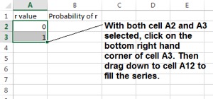
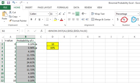
1.     Begin by entering the information in the given cells as seen on the right. Fill the series to include values 0-10 in column A.

MS Excel Screenshot

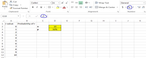
2.     Next, create cells for n and p, and enter the corresponding values. These are input cells, and it is generally good practice to visually highlight inputs within an Excel model. P can be formatted to a % by selecting the cell and clicking the % sign on the number group (circled in the below picture).

3.     Click on cell B2. (You are going to set up a formula to calculate the probability of r for an r value of 0.) Next, click on F(x) circled in the picture. Type “Binomial” in the search window and select “Go”. Click the option titled “BINOM.DIST” and select OK.

MS Excel Screenshot

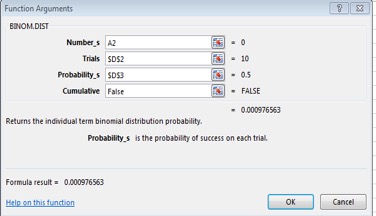
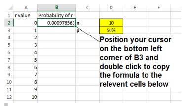
4.     Fill in the formula parameters by clicking the appropriate cell within the workbook. For trials and probability, click the desired cell, then press F4 which will add dollar signs to the cell references (Fn + F4 on some laptops). This makes the cell an absolute reference which will always be referred to when formulas are dragged.

MA Excel Screenshot

MS Excel Screenshot

MS Excel Screenshot

5.     Format the Probability of r column as the percent style by highlighting cells B2:B12 and selecting the percent style option (circled in red) Also format to 2 decimal places by clicking the increase decimal option twice (circled in blue).

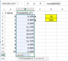
6.     The probability of all r values should add up to 100%. To check this, we can add a SUM function at the end of our probability of r column.

Select cell B13. Then type =sum(

Select cells B2:B12 and press enter. 100% should be displayed in cell B13 assuming everything was done correctly.

MS Excel Screenshot

Interpretation: Based on the table to the right, the probability of flipping 0 heads out of 10 flips is only .10% (a tenth of a percent). The value with the highest probability is flipping 5 heads at 24.61%

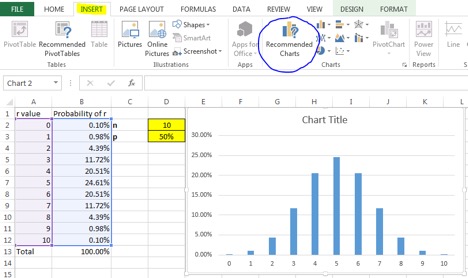
7.     Next we are going to add a clustered column chart. Highlight cells A2:B12 and select recommended charts (circled in blue) from the insert tab (highlighted in yellow). Choose the clustered column chart and select ok.

MS Excel Screenshot

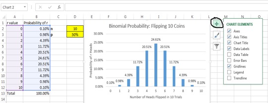
8.     Select and rename the chart title “Binomial Probability: Flipping 10 coins”. Click somewhere within the chart and select the green plus sign (chart elements). Check the boxes titled “Axis Titles” and “Data Labels”. Title the Y axis “Probability of r Heads” and the X axis “Number of heads flipped in 10 trials”.

MS Excel Screenshot

 You are finished! You have constructed a binomial distribution that shows the probability of flipping 0 to 10 heads within an experiment of 10 flips. Here are a few additional things to note:

·       Our distribution is completely symmetrical. As you can see, the probability of both 4 and 6 heads, 3 and 7 heads etc. are identical. This is because the probability of success (flipping heads) is 50%. Our distribution would be skewed if p was equal to something other than 50%.

·       The Excel model you created can be modified to change either p or n. Try different values for p to see how the distribution changes. Note that our model is set up to only function for n<=10, The chart will continue to display for n = 10 even when n is decreased in the model.