MATLAB: An Introductory Course
The Basics
What is MATLAB

MATLAB is a high-performance interactive software created by MathWorks. It is primarily used for numerical computation, matrix manipulations, plotting of functions, the application of algorithms, the creation of user interfaces and interacting with programming languages such as C, C++, and Java. You can import data into MATLAB from files, applications or external devices, and then analyze it through engineering or mathematical functions, plots and visualizations. MATLAB is available in both commercial and academic versions with new upgrades released biannually.
MATLAB is one of the top leading tools used in the engineering and scientific industries, and many job postings will specify that the employee have a strong understanding of the software. Being fluent with MATLAB is essential for working in chemical, civil, electrical and mechanical engineering. The MATLAB language supports the vector and matrix operations that are essential for engineering and science students. Students will use MATLAB for:
· Math and computation
· Algorithm development
· Modeling and prototyping
· Data analysis and visualization
· Application development
· Graphical User Interface (GUI) building
The Desktop/Interface
The general MATLAB interface will appear once you launch the software. It looks like this:
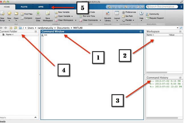
| 1 |
Command Window |
| 2 |
Workspace Browser |
| 3 |
Command History Window |
| 4 |
Current Folder Browse |
| 5 | Toolstrip |
1. Command Window
The main window for the MATLAB desktop is the Command Window and this is where you will be entering most of your data and calculations.
Tip: To determine the number of columns and rows that you can display in your Command Window, given its current size, type
get (0, ‘CommandWindowSize’)
Adjusting the size of the Command Window will change to number of columns and rows that can be displayed.
2. Workspace Browse
The Workspace Browser displays all the variables that you currently have stored in memory and their corresponding values. For example, if you type:
UMD = 1
The variable UMD will appear in the Workspace Browser with its value of 1. If you want the variable UMD to equal a different value, such as 2, then all you have to do is type:
UMD = 2
And MATLAB will overwrite the variable.
In case you forgot what value you assigned the variable, just type the variable name in the command window and hit enter.
3. Command History Window
Located below the Workspace Browser is the Command History Window. This window stores all the commands that you have entered in the Command Window. What is useful about this window is that it allows you to drag-and-drop commands: allowing you to execute the command as it is, or to edit it and execute a slightly different command.
Tip: An even faster way of accessing previously used commands is by hitting the up arrow while in the Command Window.
4. Current Folder Browser
To the left of the Command Window is the Current Folder Browser or Window. This window contains a list of files that are in your current directory. When you first launch MATLAB a folder will automatically be created for you, and you should make sure to label it according to the assignment or project you are working on.
For PC users:
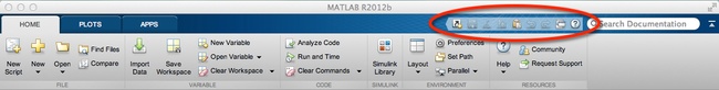
5. MATLAB Toolstrip
The MATLAB Toolstrip was a new addition in version 2012B, and it is an organized way of presenting available functionality through tabs. The components found in the Toolstrip used to be available in menus and toolbars. The basic version of MATLAB comes with the Home, Plots and Apps tabs. The light blue bar located in the upper right corner of the Toolstrip is the Quick Access Toolbar, which provides single click access to the Toolstrip functionality you use most often.
The following is a link to a MATLAB Central article discussing the different options available with the Toolbar.
MATLAB as a Calculator
MATLAB can perform basic calculations such as those you perform on a calculator. The following list is examples you should try and enter into the Command Window:
· 2+4
· 7-4
· 4*3
· 25/5
· 2^3
Trigonometry
MATLAB can be used to perform more complex calculations, such as this trigonometry function:
· sin(4*pi) + exp(-3/2)
o ans = 0.2231
It is important to remember that:
1. MATLAB has pre-defined constants; such as π may be typed pi.
2. You must type all arithmetic operations – sin(4*pi) cannot be typed sin(4pi)
Complex Numbers
Complex numbers in MATLAB contains two parts: a real part and an imaginary part. The imaginary part is declared by using ‘i’ or ‘j’. An example of this would be:
· Y = 1 + i
o Ans = 1.0000 + 1.0000i
There are several operations that create complex numbers in MATLAB. The following video will demonstrate some of these operations.
Variables
A variable is a value that may change within the scope of a given problem or set of operations. It is the opposite of a constant. In MATLAB variables allow us to reference complex and changing data. Variable can reference different data types such as scalars, arrays, vectors and matrices. Variable names must consist of a letter, which is case sensitive: meaning M and m are not the same variable.
Users can view their variables in their Workspace Browser or by using the whos command in the Command Window. By using the whos command you can also have access to the size and type of the variables.
Arrays are lists of numbers or expressions arranged in horizontal and vertical rows. A single row or column is called a vector. An array with a rows and b columns is called a matrix of size a*b.
Remember to use square brackets to denote a vector or matrix, and spaces to denote columns.
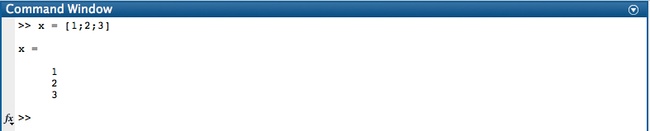
The semicolon is used to separate columns.
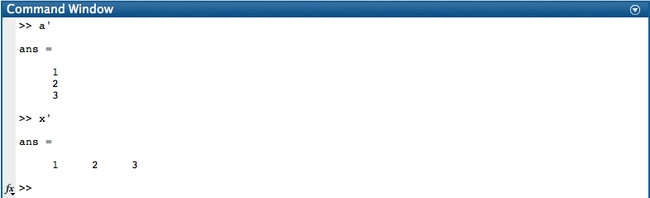
The single quotation mark ‘ transposes arrays, meaning the rows and columns are interchanged so that the first column becomes the first row.
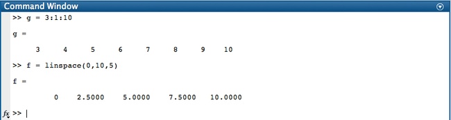
A range can be created using the colon. In the image 3:1:10 tells MATLAB to create a range that starts at 3 and goes up in steps of size 1 until 10. The linspace function also creates ranges. In the image linspace(0,10,5) is telling MATLAB to create a range between 0 and 10 with 5 linearly spaced elements.
MATLAB is a great tool for working with matrices, and was originally designed with the idea of specifically working with matrices, hence the name Matrix Laboratory. But to perform multiplication, division and exponentiation one must use the dot operator, which can be a little tricky for some students.
The dot operator is placed right before the multiplication symbol, .*, the division symbol, ./, or the exponentiation symbol, .^, in order to perform an element-by-element calculation, also known as an array operation. By not placing the dot before the arithmetic operator MATLAB will think you want the matrix version of the operator.
Tip: In order to multiply or divide two matrices they must have the same number of columns and the same number of rows.
The following video shows the dot operator in use.
If you need a quick refresher on the difference between matrix operations versus array operation, please take a look at the following pdf.
In order to access a certain element or section of a matrix one must use the (row, column) function. For example if we have the following matrix:
x = [2 4 6 8; 10 12 14 16]
but we only want to examine the 14, we would type the following in the Command Window:
x(2,3)
If we want to examine all the columns in the second row, we would use the : to indicate we want the whole column and not just a single element in that column, so we would type:
x(2,:)
The same works for rows. If we want to examine all the rows in the second column, we would type the following in the Command Window:
x(:,2)
Please watch the following video to further see how to index arrays in MATLAB
Linear Equations
MATLAB allows you to easily solve a series of linear equations. Take the following series:
7x = 2y-4z+12
4y+2z = 4x+20
2x+5y-8z = 8
The first step in the process is to re-arrange these equations so that the unknown quantities are on the left and the known quantities are on the right.
7x-2y+4z = 12
-4x+4y+2z = 20
2x+5y-8z = 8
These equations are know in the form ax=b, where a is a matrix of all the unknown coefficients.
a = 7 -2 4
-4 4 2
2 5 -8
x represents the vector of the unknowns,
x = x
y
z
and b is a vector containing the constants.
b = 12
20
8
The following video shows how you would solve this system of linear equations in MATLAB.
Tip: The left division operator (\) is used to solve equations of the form ax = b.
Plotting & Visualization
Fundamentals
MATLAB is a great tool for making both 2D and 3D plots. It is important to remember that MATLAB allows the user to create plots in various file formats, such as EPS (Encapsulated PostScript), PDF (Portable Document Format) and JPEG (Joint Photographic Experts Group). This means you can easily attach any of your plots to your assignments.

Plotting will involve using specific commands, which will depend on the type of plot you want to produce. If you happen to forget the specific command you need, you can resort to the following help options:
· help graphics – for general graphics commands
· help graph2d – for two-dimensional graphing
· help graph3d – for three-dimensional graphing
· help specgraph – for specialized graphing commands
2D Plotting
The command you will use the most for plotting graphs is plot(x,y), where x and y are vectors containing the x and y coordinates of the data you are plotting. When using the plot command you must keep the following points in mind:
· The vectors containing the x and y data must be the same length.
· The plot command can plot multiple sets of data on the same axes. An example would be plot(x1,y1,x2,y2).
The following video shows the plot command in use:
Another option for creating a simple plot would be to use the ezplot command. For example, we want to create a plot representing a parabola on the interval [-2,2]
f(x) = x^2, -2≤x≤2
We would simply use the ezplot command as such:
ezplot(‘x^2’,[-2 2])
The first input is a string describing the function, while the second input is the interval of interest in the graph. This second input is optional.
Watch the following YouTube clip if you are still unclear about the basic concept of plotting in MatLab
Plot Editing
The simplest way to edit a plot is by using the Plot Edit Toolbar. To access it you must go to your plot, click on view, and then select Plot Edit Toolbar. You can also type plotedit in the Command Window and hit enter.
Image: Insert image of plot edit toolbar.
You can cut, copy, paste, move, and resize the plot. Using specific additional commands allows you to further customize your plot. Please refer to the attached PDF file for some examples of such customizable plot commands.
The following commands are important for labeling and formatting your plot:
· Xlabel(‘text as string’) – creates a description on your x-axes
· Ylabel(‘text as string’) – creates a description on your y-axes
· Title(‘text as string’) – a title will be added to your plot
· Text(x,y,’text as string’) – a text label will be placed in your plot
· Legend(‘string 1’, ‘sting 2’,…) – this places a legend on your plot
The following video shows a plot being created using some of these commands:
Selecting the Type of Plot
1. Vertical Bar Plots – bar(x,y):
yr = [1988:1994];
sle = [8 12 20 22 18 24 27];
bar(yr,sle);xlabel(‘Year’);
ylabel(‘Sales(Millions)’);
2. Horizontal Bar Plots – barh(x,y):
yr = [1988:1994];
sle – [8 12 20 22 18 24 27];
barh(yr,sle,’r’);
xlabel(‘Year’);ylabel(‘Sales(Millions)’);
3. Stairs Plots – stairs(x,y):
K = 1:5;pmf = [1/4 ¼ ¼ 1/8 1/8];
Cdf = cumsum(pmf);
Stairs(k,cdf);
4. Stem Plots – stem(x,y):
5. Pie Plots – pie(x):
6. Histograms – hist(y,M)
Plotting Graphs - MATLAB Documentation
3D Plotting
MATLAB is a great tool for producing three-dimensional plots, such as curves, helixes, points, lines, volumes and general 3D surfaces. The plot function becomes plot3(x,y,z).
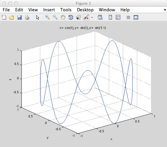
Curves
To plot 3D curves you will use the ezplot3 function. The syntax for producing a 3D curve is:
ezplot (x,y,z)
ezplot3 (x,y,z,[tmin, tmaz])
ezplot3 (…'animate')
3D Surfaces
Thee-dimensional plots can be made using two different types of surfaces: mesh and surf. The mesh surface produces a transparent grid while the surf surface produces a shadow grid. The mesh syntax is as follows:
mesh (x.y.z)
mesh (z)
mesh (…c)
mesh (…'PropertName', PropertyValue, …)
mesh (axeshandles, …)
h = mesh (…)
The colour of the mesh grid is determined by z and it is proportional to surface height. If x and y are vectors, length(x) = n and length(y) = m, where [m.n] = size(z). Mesh(z) draws a wireframe mesh using x = 1:n and y = 1:m, where [m,n] = size(z). If x.y and z are matrices, they must be the same size as c.
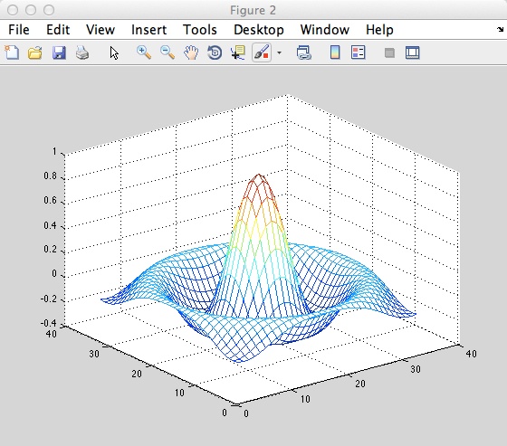
The following is an example of a mesh surface plot:
figure;
[x,y] = meshgrid (-8:.5:8);
R = sqrt (x.2 + y.2) + eps:
Z = sin(R)./R;
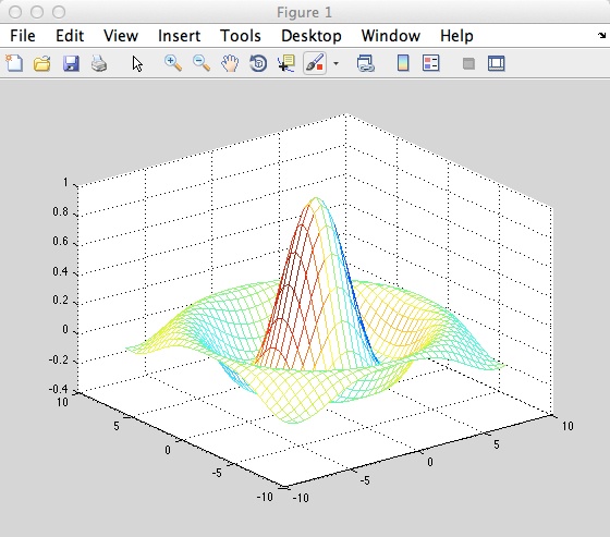
Adding the following lines will change the colour for the mesh function:
C = gradient (Z);
figure;
mesh (x,y,Z,C);
You must use the surf function to create a 3D shaded surface plot. The surf syntax is as follows:
surf (Z)
surf (Z,C)
surf (X,Y,Z)
surf (X,Y,Z,C)
surf (…'PropertyName', PropertyValue)
surf (axes handles,…)
h = surf (…)
surf(z) creates a three-dimensional shaded surface from the z components in matrix z, using x = 1;n and y = 1:m, where [m,n] = size(z). The height, z, is a single-valued function defined over a geometrically rectangular grid, z specifies the colour data, which is proportional to the surface height.
The following is an example of a sphere with the surf surface:
k = 5;
n = 2K - 1;
[x,y,z] = sphere (n);
c = hadamard (2k);
surf (x,y,z,c);
colormap ([1 1 0: 0 1 1])
axis equal
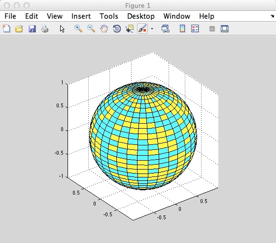
It is important to remember that the surf plot does not accept complex inputs.
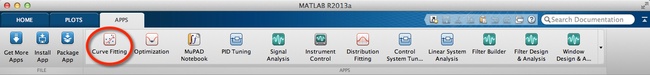
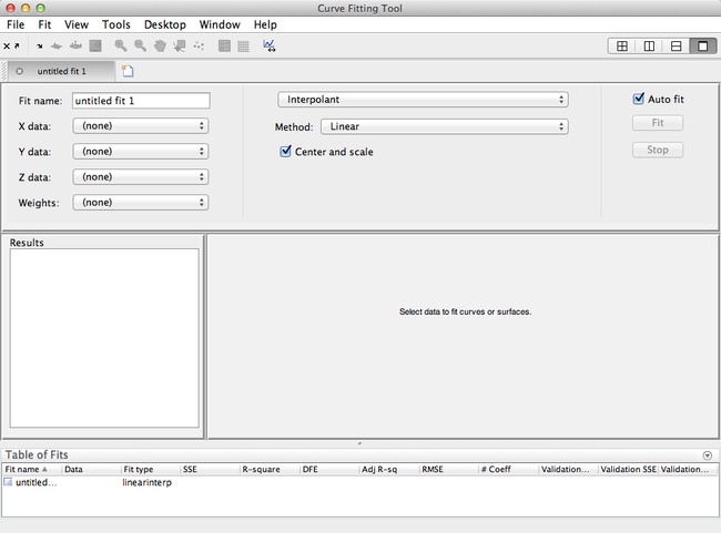
Curve Fitting Toolbox
The curve fitting toolbox is located under the Apps tab in the tools trip. It provides the user with many different options for fitting curves and placing trend-lines to the data being represented. Some of the tools that can be found are linear and nonlinear regression, splines and interpretation, and smoothing. Once you have found the correct fit, you can have MATLAB calculate the correct equation for the data.
The following video shows a general overview of all the tools available through the curve fitting toolbox:
Scripts & Functions
Scripts
When talking about scripts in MATLAB, the main focus will be on M-Files. Script m-files (.m file extensions) come in handy when you are trying to solve complicated problems. Script files allow you to easily repeat a set of commands, while only really changing one variable each time. They also allow you to document a specific sequence of actions, which might be hard to remember by oneself.
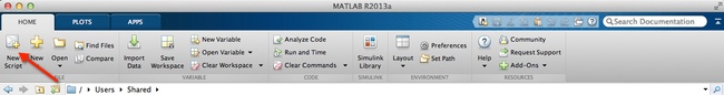
The first step in creating a new script is by clicking on the New Script tab located on the Toolstrip.
We should review some useful tips before we launch right into an example script.
- Remember to put in comments into your script files to ensure you or someone else will understand the logic behind your script. A comment is always placed following the percent sign (%). The percent sign tells MATLAB not to run the line as a command.
- Never include spaces when naming your script file. If you want to place a space you must use the underscore symbol (_). Names should not begin with a number or be names of pre-existing functions.
- You should remember to use the clear all or clc commands for your first line in your script and you should clear up the Command Window. This will make sure you are starting fresh with your new script.
Script 1
Type the following commands in the New Script window.
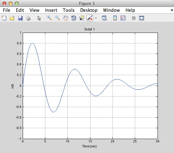
% Script 1
% This is an example of a continuous - time signal
t = exp (-.1 * t) .* sin (2/3 * t);
plot (t,x)
grid
axis ([0 30 - 1 1]);
ylabel ('x(t)')
xlabel ('Time(sec)')
title ('Script 1')
Script 2
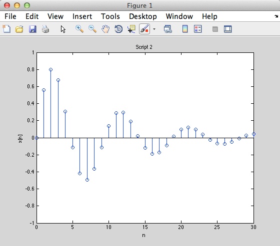
% Script 2
n = 0: 30;
x = exp (-.1 * n) . * sin (2/3 * n);
stem (n, x)
axis ([0 30 - 1 1]);
ylabel ('x[n]')
xlabel ('n')
title ('Script 2')
Script 3
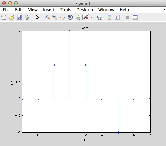
% Script 3
n = -2: 6;
x = [0 0 1 2 1 0 -1 0 0];
stem (n, x);
xlabel ('n')
ylabel ('x[n]')
title ('Script 3')
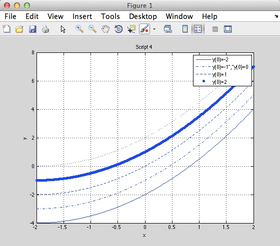
Script 4
% Script 4
x = -2 : .01 : 2;
c = -2; plot (x, x.2/2 + 2 * x + c, ' -')
hold on
c = -1; plot (x, x.2/2 + 2 * x + c, '-.')
c = 0; plot (x, x.2/2 + 2 * x + c, ' - -')
c = 1; plot (x, x.2/2 + 2 * x + c, ' .')
c = 2; plot (x, x.2/2 + 2 * x + c, ' :')
grid on
xlabel ('x')
ylabel ('y')
title ('Script 4')
legend ('y(0) = -2',' y(0) = -1'.' y(0) = 0,' y(0) = 1'.' y (0) = 2')
Final Tips
Most m-file scripts will only be used for a particular project or assignment. But if you organize your m-files and write them in a very easy to understand way, then they can be re-used for any future work. The following tips will help you create excellent scripts:
- The beginning of a script should begin with a % that identifies what the script does and the date that the script was written or last revised.
- Use comments throughout the script to make sure the program can be read by someone else.
- Use white space to break apart your program; which makes it easier to read.
- Remember to use fleas all and clc commands at the start of your script.
Functions
M-files do not always have to come in the form of scripts; they can also be in the form of Function Files. What makes functions different is that they are only available for the function itself, meaning they are only local to the function and it’s argument. Two examples of simple functions in MatLab are sqrt(x) and log(x), where the sqrt and log represent the function, and the (x) represents the individual arguments. This is different from script files because any variable you define will exist in the Workspace and can be used by other commands. With time you will become comfortable creating your own functions, which will allow you to perform specific tasks at a quicker pace.
Syntax for Functions

- The first line begins with the word function, and is mandatory because it informs the program that the m-file is a function file.
- The output variables are shown on the left hand side of the equals sign, and the input variables are shown on the right.
- The name of the function file must be on the right side of the equals sign and must match the name used to save the file.
- Remember to include comments after the function definition line to help explain your reasoning and logic for the m-file.
The following video shows the creation of a simple function file. The function is of the equation y = x.^2 + cos (x).

- It is important to remember that the . is placed after the x in order to vectorize the function. If you make the function y = x^2 + cos(x), it will not be compatible with vectors and matrices.
- Place semicolons at the end of your functions in order to avoid showing intermediate computations.
Inline Functions
The inline command allows you to quickly create simple functions. Inline functions are similar to function m-files: they accept input (which is usually numerical) and return output. The difference is that with inline functions the evaluation takes place in the current workspace, whereas function m-files operate in separate workspaces. The following is an example of an inline function in MATLAB:
' (1 + x) .^2. / (1 + x .^ 2)'
y = inline (ans .'x')
y (1) . y ([ 2 4 6])
f plot (y . [-100 100])
- The plot command will allow you to plot your inline function.
Object-Oriented Programming (OOP)
Introduction to OOP
Object-oriented programming (OOP) applies to the development of software or “objects” that have data fields (attributes that describe the object) and associated procedures known as methods. Objects are composed of two elements: data, such as numbers, strings or variables and actions such as functions. You can then combine objects or have them interact together in order to design applications and computer programs. Examples of object-oriented programming languages include Objective-C, Smalltalk, Java and C#.
Classes
One of the first distinctions you must make before trying to create programs in MATLAB is the difference between classes and objects. A class is a definition that specifies certain characteristics that all instances of the class share. These characteristics are determined by the properties, methods and events that define the class and the values of attributes that modify the behaviour of each of these class components. Class definitions describe how objects of the class are created and destroyed, what data the objects contain, and how you can manipulate this data.
Objects contain actual data for a particular entity that is represented by the class. An example to help better explain the difference is to think that a class is like a bank account, while an object is one specific bank account that includes a real account number.
The following table will help you better understand other common definitions used in MATLAB.
| Term | Definition |
| Class Definition | Description of what is common to every instance of a class. |
| Properties | Data storage for class instances. |
| Methods | Special functions that implement operations that are usually performed only on instances of the class. |
| Events | Messages that are defined by classes and broadcasts by class instances when some specific action occurs. |
| Attributes | Values that modify the behaviour of properties, methods, events, and classes. |
| Listeners | Objects that respond to a specific event by executing a callback function when the event notice is broadcast. |
| Objects | Instances of classes, which contain actual data values stored in the objects' properties. |
| Subclasses | Classes that are derived from other classes and that inherit the methods, properties, and events from those classes (subclasses facilitate the reuse of code defined in the superclass from which they are derived). |
| Superclasses | Classes that are used as a basis for the creation of more specifically defined classes (i.e., subclasses). |
| Packages | Folders that define a scope for class and function naming. |
Defining A Class
The first step to defining a class is by creating a new m-file with the same name as the class you want to create. You need to start the file with the classed keyword followed by the class name. The following line is for defining the properties and methods of the class. A special keyword called the constructor is needed to create or construct a new object, and it must have the same name as the class. the constructor can take any argument which specifies initial values for the properties, and must return one argument, the constructed object. Properties can optionally be assigned default values. If no default is specified and no value is assigned by the constructor, they are assigned the empty matrix.
The following is an example of how to create a class in MATLAB:
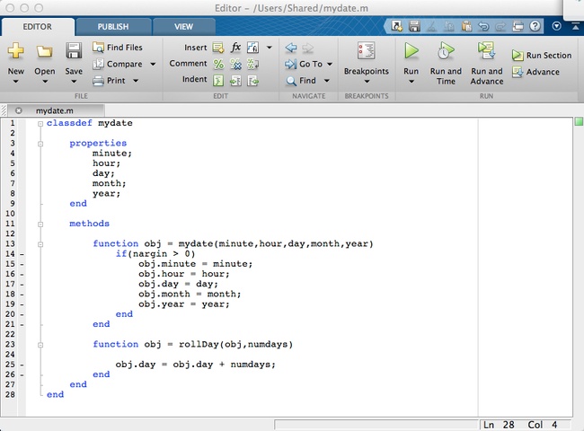
| Line | Explanation |
| classdef mydate | This is where you write a description of the class |
| function obj = mydate (minute, hour, day, month, year) | This is the class constructor |
Now that you have created the class, you can create date objects. The following two lines are examples of how you can create date objects.
d1 = mydate )0, 5, 20, 5, 1990);
d2 = mydate ();
The properties that you have just defined are public, meaning that they are accessible from outside the class. You can access and assign them using dot notion:
day = d1.day;
d1.year = 1990;
Loops
Loops allow you to alter the flow of control in your programs. They come in handy when you need to repeat exe
cuting commands. Sometimes you may want to repeat the same commands while still changing the value of a variable each time or until a certain condition is met. There are two types of loops, for and while, and both will be examined here.
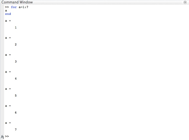
For Loops
For loops are used to repeat a command, or a set of commands, for a fixed number of times. The following is a syntax for a for loop:
for variable = f : s : t
statement
end

- Line 1 contains the for command, followed by the loop counter variable. The first expression, u, is the value of the loop counter on the first iteration of the loop, m, is the increment size, and d is the value of the loop counter on the final iteration of the loop. An example of this loop counter would be the expression n = 0:5:25, which means n = [0 5 10 15 20 25].
- Line 2 contains the body of the loop, which can be a command, or a series of commands. These commands will be executed on each iteration of the loop.
- Line 3 contains the end command that must always be included in order to close the loop
Simple For Loop
While Loops
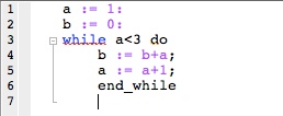
A while loop is similar to for loops in that they repeat commands. The major difference is that a while loop will continue to execute until a specified condition becomes false. The following is a syntax for a while loop:
While condition is true
statements
end
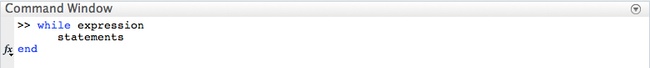
· Line 1 contains the while command, followed by a condition such as a<7. As long as the condition, a<7, remains true, the loop will continually repeat.
· Line 2 contains the body of loop, which will have a command or series of commands that will be executed on each iteration of the loop.
· Line 3 contains the end command, which must always be used at the end of the loop in order to close it.
The while loop can be used to make a more efficient algorithm. A for loop can use up lots of memory because it does not stop at a pre-determined condition like a while loop does. A better way of creating an algorithm is to have it repeat the same operations only as long as the number of steps is below some determined condition.
Simple While Loop
Branching
When a program makes a choice to do one of two (or more things) this is called branching. The three most common programming statements used to branch is the if, else and elseif. These branching statements Before getting into these three statements, we will review relational operators, which are used to help make decisions in your algorithms.
If Statement
The syntax for an if statement is:

· The first line contains the if command, followed by an expression that must return as true or false.
· The second line contains the body of the if command, followed by a series of commands that will run if the expression entered returns as true.
· The third line is the end command which closes the if statement.
Else and Elseif Statements
The syntax for an if statement which contains the else and elseif commands is:
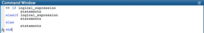
· The expression on line 3, the elseif command, will only be evaluated if the expression preceding it returns as false.
· The expressions following the else command will only be executed if all the logical expressions for the elseif and if commands return as false.
Additional Resources
Official MATLAB/MathWorks
MATLAB Central: A database of resources dealing with MATLAB. Including MATLAB Answers, Newsgroup, File Exchange and Tutorial Videos.
MathWorks Support: This support page includes Documentation Center, User Community, Technical Solutions, Bug Reports and Downloads.
Books
MATLAB (3rd ed) - A Practical Introduction to Programming and Problem Solving: This book assumes the user has no pre-existing knowledge of programming, and thus is great for beginners. Topics include variables, assignments, loops, and gives a solid foundation for how MATLAB can be applied to engineering.
MATLAB - An Introduction with Applicants: This book does a great job at providing a good array of problems, and each come with step-by-step instructions on how to complete them.
Essential MATLAB for Engineers and Scientists (5th ed): This book is great because it covers program and algorithm development, with a focus on engineering and science students.
Plotting
Plotting Functions: Explains all the elements needed to created a specific plot, such as specifying line style, colour, data points and markers.
Scripts & Functions
MATLAB Functions: Discusses the creation of m-files and assigning input and output parameters.
Examples of MATLAB Functions: This is a great resource that shows you how to create all the different types of functions in MATLAB.
Object-Oriented Programming
Object-Oriented Programming for MATLAB: Provides a breakdown of how to develop computer applications in MATLAB.
Developing Classes Overview: This is a video that discusses how to create classes.