WP.4.1 DISCRETE PROBABILITY DISTRIBUTIONS

[WP.4.1]

WHITE PAPER TOPIC: DISCRETE PROBABILITY DISTRIBUTIONS

A probability distribution arises when the possible outcomes from a situation are listed along with each outcome’s probability of occurring. Take for example the number of boats sold by boat salesman Johnny Smith on any given day. A possible probability distribution is shown in the following table:

The table shows that Johnny Smith sells between 0 and 4 boats on a given day, with 2 boats being the most common value at 40%. The probability column can also be expressed as percentages. Note that the sum of the probabilities must always add up to 1 or 100%.

This particular type probability distribution is called a Discrete Probability Distribution: Meaning there is a finite number of possible outcomes (in our case, we have the values 0 through 4 boats where we cannot sell a partial boat).

There are a few interesting things we can do with discrete probability distributions such as calculating the Mean, Variance, and Standard Deviation.

I.               MEAN OF A DISCRETE PROBABILITY DISTRIBUTION

The formula for the mean (also known as expected value) of a discrete probability distribution is computed by the formula:

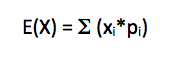
Formula for calculation of Mean for a Discrete Probability Distribution

Where:

E(X) = Expected Value

x_i = Each discrete outcome

p_i = Probability of each outcome

The symbol on the right hand of the equation is a capital sigma, which is also known as summation. So in words, the expected value is = to the sum of each discrete outcome multiplied by the corresponding probability. The expected value for Johnny Smith’s boat sales can be calculated as follows:

(0*.05) + (1*.2) + (2*.4) + (3*.25) + (4*.10) = 2.15 boats

This represents the average, or expected value of our distribution. Note that this value might not necessarily be one of our possible discrete outcomes. In our example, Johnny could not possibly sell 2.15 boats in a given day; this value serves as an average quantity of boats sold.

II.              VARIANCE AND STANDARD DEVIATION OF A DISCRETE PROBABILITY DISTRIBUTION.

Although a useful measure of an average for the distribution, the expected value fails to describe how spread out the data is. The Variance helps us solve this problem. Variance can be calculated by the formula:

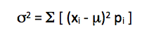
Formula for calculation of Variance for a Discrete Probability Distribution

Where:

x_i = Each discrete outcome

p_i = Probability of each outcome

sigma² = Variance

mu = Mean or Expected Value

In words, the variance can be computed by taking the sum of the squared difference from each discrete outcome to the mean, multiplied by each corresponding probability.

Revisitng Johnny Smith and his boat sales, the variance is calulcated as follows:

[(0-2.15)² * .05]+ [(1-2.15)² * .2] + [(2-2.15)² * .4] + [(3-2.15)² * .25] + [(4-2.15)² * .1] = 1.0275

A comparison of variances among separate probability distributions allows us to determine how spread out the data is. A larger variance would mean we have a lot of data values far from the mean, whereas a low variance would suggest the data is clumped together very close to the mean.

The Standard Deviation of a discrete probability distribution is found simply by taking the square root of the variance. So in our example √1.0275 = 1.0137 standard deviation.

III.            ADDITIONAL PROBLEMS

Problem 1: What is wrong with this probability distribution?

Problem 2: True or False: A discrete probability distribution contains a finite number of outcomes, with a corresponding probability assigned to each outcome.

Problem 3: True or False: The mean or expected value of a discrete probability distribution must be one of the possible discrete outcomes.

Problem 4: Find the missing probability in the following probability distribution

Problem 5: Farmer Fred sells his potatoes is three different size bags: A 5 lb, a 10 lb, and a 15 lb bag. Based on his past experience, Fred has created the following discrete probability distribution related to sales of each bag of potatoes given that a customer has purchased a bag of potatoes.

Calculate the mean, variance and standard deviation for the sale of Farmer Fred’s potatoes

Problem 6: Find the missing X value in the following probability distribution given the expected value is 272.1

Problem 7: Artsy Anne knits custom scarves to sell online. She typically waits until she has an order and then begins knitting the scarf. The following probability distribution shows how many scarves Artsy Anne has orders for in any given week and the corresponding probabilities:

Calculate the mean, variance, and standard deviation for the quantity of scarf orders Artsy Anne receives in a week.

Problem 8: The discrete probability distribution for rolling a 4 sided die is given as follows:

Calculate the mean, variance, and standard deviation.

SOLUTIONS

Problem 1:           The sum of the probabilities do not add up to 1

Problem 2:           True

Problem 3:           False

Problem 4:           0.2

Problem 5:           Mean: 8 Potatoes

                             Variance: 11

                             Standard Deviation: 3.32

Problem 6:           266

Problem 7:           Mean: 4.55

                             Variance: 1.0475

                             Standard Deviation: 1.0235

Problem 8:           Mean: 2.5

                             Variance: 1.25

                              Standard Deviation: 1.118